Data analysis with the tidyverse
Dr Gregorio Alanis-Lobato - AG Andrade (galanisl@uni-mainz.de)
1 Intro and Overview
1.1 Introduction
The advent of high-throughput technologies, like RNA-Seq and ChIP-Seq, has resulted in a flood of huge amounts of data in the life sciences. In consequence, computational and statistical skills are becoming a key part of the life scientist’s curriculum.
The goal of this module is to give you a foundation in the most important tools for data analysis in R. You can then complement and expand your knowledge on your own in order to perform more complex analyses.
This module borrows materials and concepts from the book R for Data Science by Garret Grolemund and Hadley Wickham. R for Data Science is a great place to start if you want to learn more about data analysis with R.
1.2 Pre-requisites
1.2.1 R and RStudio
Make sure that R and RStudio are installed in your computer.
1.2.2 The tidyverse and ggvis
As the title of the module suggests, it is based on a powerful set of packages for data manipulation and visualisation known as the tidyverse. We will also need the ggvis package to generate interactive figures and explore our data. So, make sure that both have been installed in your R environment.
1.3 Overview
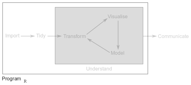
In most data analysis projects you will have to do the following:
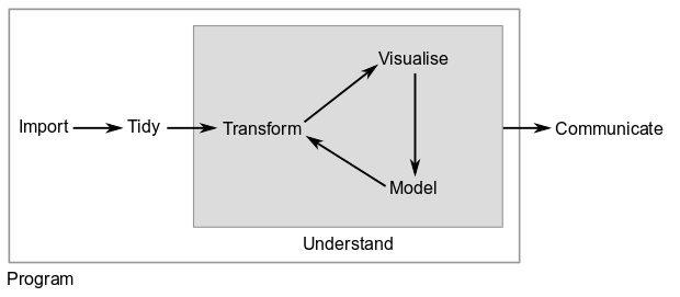
The tidyverse set of packages include functions to tackle each one of the parts of the data analysis process.
1.3.1 Import
The first step in data science is to import your data into R in order to manipulate it with R functions. This means that you will take data stored in a file, database or website and load it into a variable in R. These datasets can be the output of a genomics project, the result of a survey, measurements done in the lab, etc.
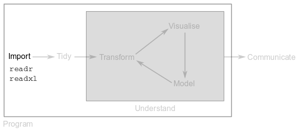
In this module, you will use functions from the readr and readxl packages to load data into R.
1.3.2 Tidy
Second, you will have to tidy up your data. Briefly, in a tidy dataset each row is an observation or a sample and each column is a variable. If your data is tidy and has a consistent structure, you will be able to use it seamlessly throughout the tidyverse.
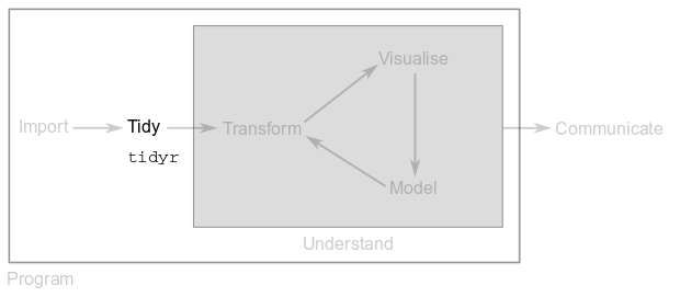
In this module, you will use functions from the tidyr package to tidy up your data.
1.3.3 Transform
Once your data is tidy, often times you need to transform it. Common transformations include normalisation, the creation of new variables from existing ones (e.g. convert from inches to centimetres) or the computation of summary statistics (e.g. means and counts).
In this module, you will use functions from the dplyr package (the d comes from data-frame and plyr from “pliers”, the pincers for gripping small objects or bending wire) to perform data transformations.
1.3.4 Visualise and model
Armed with tidy data that has the variables you need, you are ready for knowledge generation. Good data graphics will show you things that you didn’t know about the data, they will also show you things you didn’t expect, raise more questions or tell you that you’re asking the wrong questions.
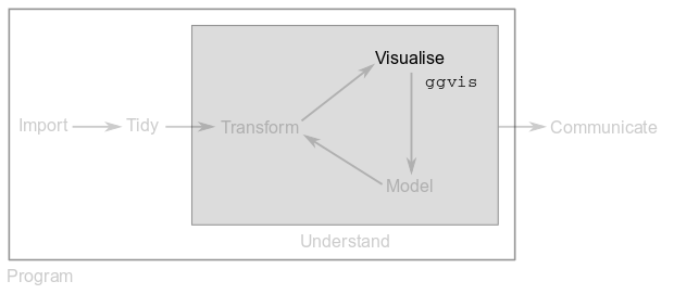
In this module, you will generate interactive plots to gain a better understanding of your data. This will be done with functions from the ggvis package.
Models are complementary to visualisations. Models are mathematical representations of a system that are often derived from precise data analyses and observations. Models are key to making predictions that can be later tested in the lab.
Even though there are powerful tools in R for data modelling, in this module you will only propose simple models based on visualisations.
It is important to stress that visualisation and modelling will often derive in new questions and hypotheses that will bring you back to the data transformation step. With new variables and stats, you can visualise again and fine tune your model.
1.3.5 Program
Surrounding all the above steps is programming, a critical part of any data analysis project. You don’t need to be an expert programmer to analyse data, but programming skills allow you to automate common tasks and solve new problems more easily.
There are hundreds of programming languages out there, but R and its rich collection of packages, functions and data are particularly useful when it comes to doing statistics and data analysis.
1.3.6 Communicate
Cool graphics and precise models are of no use if you cannot communicate your results to others. Communication of methods and results can be done via oral or poster presentations, theses, scientific articles, reports, etc.
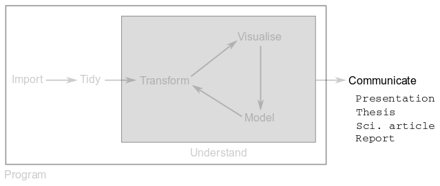
There are tons of tools for communication of data analyses, from PowerPoint or Word to web pages and R Markdown. These interactive notes have been written with the latter.
1.4 Example data analysis pipeline
To motivate your interest for data analysis and give you a glimpse of how easy it is to do it in the tidyverse, the following lines will guide you through an example project aimed at automating the classification of iris flowers.
The example will go through all the steps covered above and highlight some of the functions that you will learn and use in this module. Don’t freak out about the code or the data analysis itself. Everything will be explained in more detail in the following Parts.
1.4.1 The iris flower dataset
The iris flower dataset was collected by Edgar Anderson, an American botanist, in the 1920s. This data was used by statistician Ronald Fisher to demonstrate statistical methods of classification.
The original dataset contains 150 samples from three iris species. You are going to work with a reduced version with only 100 samples from two species: Iris setosa and Iris virginica.
For each sample, Anderson recorded the sepal length and width, as well as the petal length and width:
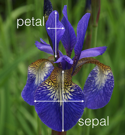
An iris flower and Anderson’s measurements (taken from Kaggle.com)
Given an iris flower, is it possible to classify it as setosa or virginica based on these measurements?
Before starting our analysis, we need to load the tidyverse and ggvis packages:
library(tidyverse)## ── Attaching packages ──────────────────────────────────────────────────── tidyverse 1.2.1 ──## ✔ ggplot2 2.2.1 ✔ purrr 0.2.4
## ✔ tibble 1.4.2 ✔ dplyr 0.7.4
## ✔ tidyr 0.8.0 ✔ stringr 1.3.0
## ✔ readr 1.1.1 ✔ forcats 0.3.0## ── Conflicts ─────────────────────────────────────────────────────── tidyverse_conflicts() ──
## ✖ dplyr::filter() masks stats::filter()
## ✖ dplyr::lag() masks stats::lag()library(ggvis)##
## Attaching package: 'ggvis'## The following object is masked from 'package:ggplot2':
##
## resolution1.4.2 Importing the iris dataset
There is a file called iris.tsv in your folder datasets. The file extension tells us that this is a “tab-separated value” type of file and the readr package from the tidyverse has function read_tsv to import them into R:
ir <- read_tsv("datasets/iris.tsv")## Parsed with column specification:
## cols(
## ratio_sl_sw = col_character(),
## ratio_pl_pw = col_character(),
## species = col_character()
## )Variable ir now contains the iris flower data table.
ir## # A tibble: 100 x 3
## ratio_sl_sw ratio_pl_pw species
## <chr> <chr> <chr>
## 1 5.1/3.5 1.4/0.2 setosa
## 2 4.9/3 1.4/0.2 setosa
## 3 4.7/3.2 1.3/0.2 setosa
## 4 4.6/3.1 1.5/0.2 setosa
## 5 5/3.6 1.4/0.2 setosa
## 6 5.4/3.9 1.7/0.4 setosa
## 7 4.6/3.4 1.4/0.3 setosa
## 8 5/3.4 1.5/0.2 setosa
## 9 4.4/2.9 1.4/0.2 setosa
## 10 4.9/3.1 1.5/0.1 setosa
## # ... with 90 more rows1.4.3 Tidying the iris dataset
Remember that tidy datasets report each sample in its own row and each variable in its own column. The iris dataset reports sepal length and width and petal length and width as ratios in columns ratio_sl_sw and ratio_pl_pw, respectively. We can tidy up this table with function separate from package tidyr:
ir <- ir %>%
   separate(col = ratio_sl_sw,
            into = c("sepal_length", "sepal_width"), sep = "/") %>%
   separate(col = ratio_pl_pw,
            into = c("petal_length", "petal_width"), sep = "/")
1.4.4 Transforming the iris dataset
ir## # A tibble: 100 x 5
## sepal_length sepal_width petal_length petal_width species
## <chr> <chr> <chr> <chr> <chr>
## 1 5.1 3.5 1.4 0.2 setosa
## 2 4.9 3 1.4 0.2 setosa
## 3 4.7 3.2 1.3 0.2 setosa
## 4 4.6 3.1 1.5 0.2 setosa
## 5 5 3.6 1.4 0.2 setosa
## 6 5.4 3.9 1.7 0.4 setosa
## 7 4.6 3.4 1.4 0.3 setosa
## 8 5 3.4 1.5 0.2 setosa
## 9 4.4 2.9 1.4 0.2 setosa
## 10 4.9 3.1 1.5 0.1 setosa
## # ... with 90 more rowsNote that the width and length columns in the tidied iris dataset are of type character instead of numeric. If we want to compute means or other statistics on this table, we need to transform these columns into the appropriate type. We can do this with function mutate from package dplyr:
ir <- ir %>%
   mutate(sepal_length = as.numeric(sepal_length),
          sepal_width = as.numeric(sepal_width),
          petal_length = as.numeric(petal_length),
          petal_width = as.numeric(petal_width))
1.4.5 Visualising the iris dataset
Let’s now plot histograms for each flower feature to see if there’s one that can be used to classify the two iris species:
ir %>%
   group_by(species) %>%
   ggvis(x = ~sepal_length, fill = ~species) %>%
layer_histograms(width = 0.15)ir %>%
group_by(species) %>%
ggvis(x = ~sepal_width, fill = ~species) %>%
layer_histograms(width = 0.15)ir %>%
group_by(species) %>%
ggvis(x = ~petal_length, fill = ~species) %>%
layer_histograms(width = 0.15)ir %>%
group_by(species) %>%
ggvis(x = ~petal_width, fill = ~species) %>%
layer_histograms(width = 0.15)1.4.6 Modelling
Thanks to the above plots, we know that we can use petal length and width to differentiate between a flower from the species Iris setosa and the species Iris virginica. Under the assumption that we’re only dealing with flowers from these two species, let’s use our observations to propose a simple model for iris flower classification:
# Note that this is not valid R code!

Given a flower x

if (x$petal_length <= 3 && x$petal_width <= 1){
   x is Iris setosa
}else{
   x is Iris virginica
}