2 Import and the tibble
2.1 Importing data into R
In Part 1, you saw that the first step in any data analysis pipeline is importing your tables into R. You do this to take advantage of R’s functions, which simplify the manipulation of your data.
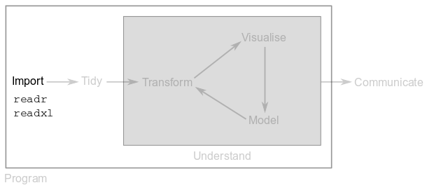
There are two packages in the tidyverse that make data import into R a matter of a single line of code.
Package readr provides functions to import data stored in plain-text files, such as “comma-separated value” or “tab-separated value” files.
Package readxl provides functions to import data stored in Microsoft Excel files. These functions also let you import from specific sheets or ranges within the Excel file.
2.2 Importing from plain-text files
To demarcate the content of each cell in a file, people use special characters like commas, tabs, pipes, etc. The extension of plain-text files is often a good hint of what delimiter has been used. For example, csv files use “commas” as the delimiter, whereas tsv files use “tabs”. Nevertheless, you can find csv or tsv files that are delimited with different characters.
The first step in data import is locating the file in your computer or in a remote location. The most important parameter for readr’s functions is the path to the file of interest.
In this part, you are going to import files located in folder datasets. Packages tidyverse and readxl must be loaded.
2.2.1 Importing a tsv file
Let’s start by learning how to import a tsv file:
who_ref <- read_tsv("datasets/who_ref.tsv")## Parsed with column specification:
## cols(
## country = col_character(),
## year = col_double(),
## cases = col_integer(),
## population = col_integer()
## )who_ref## # A tibble: 6 x 4
## country year cases population
## <chr> <dbl> <int> <int>
## 1 Afghanistan 1999. 745 19987071
## 2 Afghanistan 2000. 2666 20595360
## 3 Brazil 1999. 37737 172006362
## 4 Brazil 2000. 80488 174504898
## 5 China 1999. 212258 1272915272
## 6 China 2000. 213766 12804285832.2.2 Importing a csv file
Importing a csv file is very similar:
who1 <- read_csv("datasets/who1.csv")## Parsed with column specification:
## cols(
## country = col_character(),
## year = col_double(),
## type = col_character(),
## count = col_integer()
## )who1## # A tibble: 12 x 4
## country year type count
## <chr> <dbl> <chr> <int>
## 1 Afghanistan 1999. cases 745
## 2 Afghanistan 1999. population 19987071
## 3 Afghanistan 2000. cases 2666
## 4 Afghanistan 2000. population 20595360
## 5 Brazil 1999. cases 37737
## 6 Brazil 1999. population 172006362
## 7 Brazil 2000. cases 80488
## 8 Brazil 2000. population 174504898
## 9 China 1999. cases 212258
## 10 China 1999. population 1272915272
## 11 China 2000. cases 213766
## 12 China 2000. population 1280428583Note how simple the syntax for data import is: you choose the name of a variable to store your table, use the <- operator, call the appropriate readr function and specify the location of your file.
2.2.3 Exercise 2.1
Read file datasets/andrade_lab.csv into variable al and show the content of the variable.
2.2.4 Importing a text file
If the column delimiter of a file is not obvious from its extension and the person in charge of the file didn’t provide this information, you must first figure out which delimiter was used. For example, open the following file datasets/who2.txt.
Since the delimiter is a -, we need to call read_delim to import:
who2 <- read_delim("datasets/who2.txt", delim = "-")## Parsed with column specification:
## cols(
## country = col_character(),
## year = col_double(),
## rate = col_character()
## )who2## # A tibble: 6 x 3
## country year rate
## <chr> <dbl> <chr>
## 1 Afghanistan 1999. 745/19987071
## 2 Afghanistan 2000. 2666/20595360
## 3 Brazil 1999. 37737/172006362
## 4 Brazil 2000. 80488/174504898
## 5 China 1999. 212258/1272915272
## 6 China 2000. 213766/1280428583Note that in this special case, you have to specify the delimiter using parameter delim.
2.2.5 Exercise 2.2
From its extension, file datasets/andrade_lab.tsv is supposed to be tab-separated. Read the file with function read_tsv into variable al and show its contents. What character is the delimiter in this file? Use the appropriate readr function to import this table into R.
2.3 Importing from Excel files
The syntax to import from Excel files is very similar to the one used above.By default, function read_excel imports from the first available sheet:
who_cases <- read_excel("datasets/who_split.xlsx")
who_cases
## # A tibble: 3 x 3
## country `1999` `2000`
## <chr> <dbl> <dbl>
## 1 Afghanistan 745. 2666.
## 2 Brazil 37737. 80488.
## 3 China 212258. 213766.If you want data from a different sheet, you must use parameter sheet:
who_pop <- read_excel("datasets/who_split.xlsx", sheet = "population")
who_pop
## # A tibble: 3 x 3
## country `1999` `2000`
## <chr> <dbl> <dbl>
## 1 Afghanistan 19987071. 20595360.
## 2 Brazil 172006362. 174504898.
## 3 China 1272915272. 1280428583.You can also specify a range to import from:
who_pop_99 <- read_excel("datasets/who_split.xlsx", sheet = "population",
                         range = "A1:B4")
who_pop_99
## # A tibble: 3 x 2
## country `1999`
## <chr> <dbl>
## 1 Afghanistan 19987071.
## 2 Brazil 172006362.
## 3 China 1272915272.2.3.1 Exercise 2.3
Import the list of PhD students in Andrade Lab from file datasets/andrade_lab.xlsx. Choose a variable name to store the file contents.
2.4 The tibble
Reading files with readr or readxl functions results in the creation of a variable of type tbl_df instead of R’s traditional data frame (type data.frame). This is because one of the unifying features of the tidyverse is the tibble (type tbl_df).
# Using base R function to import CSV files
who1_df <- read.csv("datasets/who1.csv")
class(who1_df)
## [1] "data.frame"# Using readr function to import CSV files
who1_tb <- read_csv("datasets/who1.csv")## Parsed with column specification:
## cols(
## country = col_character(),
## year = col_double(),
## type = col_character(),
## count = col_integer()
## )class(who1_tb)## [1] "tbl_df" "tbl" "data.frame"tibbles are data frames but they tweak some old behaviours that make our life easier when analysing data.
To start with, printing the content of a tibble shows a rich output that gives information about the data type of each column. By contrast, data frames just show the records as is:
who1_tb## # A tibble: 12 x 4
## country year type count
## <chr> <dbl> <chr> <int>
## 1 Afghanistan 1999. cases 745
## 2 Afghanistan 1999. population 19987071
## 3 Afghanistan 2000. cases 2666
## 4 Afghanistan 2000. population 20595360
## 5 Brazil 1999. cases 37737
## 6 Brazil 1999. population 172006362
## 7 Brazil 2000. cases 80488
## 8 Brazil 2000. population 174504898
## 9 China 1999. cases 212258
## 10 China 1999. population 1272915272
## 11 China 2000. cases 213766
## 12 China 2000. population 1280428583who1_df## country year type count
## 1 Afghanistan 1999 cases 745
## 2 Afghanistan 1999 population 19987071
## 3 Afghanistan 2000 cases 2666
## 4 Afghanistan 2000 population 20595360
## 5 Brazil 1999 cases 37737
## 6 Brazil 1999 population 172006362
## 7 Brazil 2000 cases 80488
## 8 Brazil 2000 population 174504898
## 9 China 1999 cases 212258
## 10 China 1999 population 1272915272
## 11 China 2000 cases 213766
## 12 China 2000 population 1280428583Also, tibbles never change the type of the inputs: while column country is of type character in who1_tb, it was imported as a factorin who1_df.
class(who1_tb$country)## [1] "character"class(who1_df$country)## [1] "factor"This is problematic because being a factor, country cannot take other values other than the ones imported. If we want to append information about a new country to our table, it will be added but as an NA:
rbind(who1_df, c("Mexico", 1999, "cases", 100))## Warning in `[<-.factor`(`*tmp*`, ri, value = "Mexico"): invalid factor
## level, NA generated## country year type count
## 1 Afghanistan 1999 cases 745
## 2 Afghanistan 1999 population 19987071
## 3 Afghanistan 2000 cases 2666
## 4 Afghanistan 2000 population 20595360
## 5 Brazil 1999 cases 37737
## 6 Brazil 1999 population 172006362
## 7 Brazil 2000 cases 80488
## 8 Brazil 2000 population 174504898
## 9 China 1999 cases 212258
## 10 China 1999 population 1272915272
## 11 China 2000 cases 213766
## 12 China 2000 population 1280428583
## 13 <NA> 1999 cases 100Since packages outside the tidyverse use data frames, you might want to coerce them to tibbles with function as_tibble:
who1_df <- as_tibble(who1_df)In addition, it’s possible for a tibble to have column names that are not valid R variable names. For example, they might not start with a letter, or they might contain unusual characters:
unusual <- read_tsv("datasets/unusual.tsv")## Parsed with column specification:
## cols(
## `:)` = col_character(),
## `with space` = col_character(),
## `2000` = col_character()
## )unusual## # A tibble: 1 x 3
## `:)` `with space` `2000`
## <chr> <chr> <chr>
## 1 smile space numberTo refer to these column names, you have to use back-ticks:
unusual$`:)`## [1] "smile"Finally, you can create your own tibbles with function tibble:
stocks <- tibble(
  year   = c(2015, 2015, 2015, 2015, 2016, 2016, 2016),
  qtr    = c(   1,    2,    3,    4,    2,    3,    4),
  revenue = c(1.88, 0.59, 0.35,   NA, 0.92, 0.17, 2.66)
)
stocks
## # A tibble: 7 x 3
## year qtr revenue
## <dbl> <dbl> <dbl>
## 1 2015. 1. 1.88
## 2 2015. 2. 0.590
## 3 2015. 3. 0.350
## 4 2015. 4. NA
## 5 2016. 2. 0.920
## 6 2016. 3. 0.170
## 7 2016. 4. 2.66