3 Tidy data
3.1 Foreword
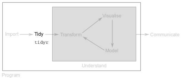
The rationale behind the tidy data philosophy is to organise the data you imported to or created in R into a consistent format. The goal is to spend less time formatting your data and more time analysing it. If your data is tidy you will be able to use it seamlessly across the tidyverse.
This part will show you how to use the functions from package tidyr to tidy up your data. As a result, data transformations and visualisations will be a real piece of cake.
Packages tidyverse and readxl must be loaded.
3.2 What is tidy data?
There are three simple and interrelated rules that make a dataset tidy:
- Each observation/sample must be reported in its own row.
- Each variable/feature describing the sample must have its own column.
- Each value must have its own cell.
Let’s import some tables from the datasets directory of your data_analysis folder and check if they fulfil the above rules.
3.2.1 Exercise 3.1
Import file datasets/who1.csv into variable who1 and show the imported data. Is the who1 dataset tidy?
3.2.2 Exercise 3.2
Import file datasets/who2.txt into variable who2 and show the imported data. Is the who2 dataset tidy?
3.2.3 Exercise 3.3
Import sheet population from file datasets/who_split.xlsx into variable who_pop and show the imported data. Is who_pop tidy?
3.2.4 Why tidy data?
Why ensure that your data is tidy? There are two main advantages:
- If you have a consistent data structure, it’s easier to learn the tools that work with it because they have an underlying uniformity. The functions in the
tidyverseall work flawlessly with tidy datasets. - Placing variables in columns allows R’s vectorised nature to shine.
The principles of tidy data seem very obvious. Unfortunately, most data that you will encounter will be untidy. There are two main reasons:
- Most people aren’t familiar with the principles of tidy data.
- Data is often organised to facilitate some use other than analysis.
This means that for most real analyses, you’ll need to tidy your data.
3.3 Spreading and gathering
When you’re in front of a dataset, the first step is always to figure out what the observations and the features that describe them are. The second step is to solve one of two common problems:
- One observation is scattered across multiple rows.
- One feature is spread across multiple columns.
To fix these problems, the tidyverse provides you with functions spread() and gather().
3.3.1 Spreading
You use function spread() for Problem 1: one observation is scattered across multiple rows. That’s exactly the problem we saw in table who1:
## Parsed with column specification:
## cols(
##   country = col_character(),
##   year = col_double(),
##   type = col_character(),
##   count = col_integer()
## )who1## # A tibble: 12 x 4
## country year type count
## <chr> <dbl> <chr> <int>
## 1 Afghanistan 1999. cases 745
## 2 Afghanistan 1999. population 19987071
## 3 Afghanistan 2000. cases 2666
## 4 Afghanistan 2000. population 20595360
## 5 Brazil 1999. cases 37737
## 6 Brazil 1999. population 172006362
## 7 Brazil 2000. cases 80488
## 8 Brazil 2000. population 174504898
## 9 China 1999. cases 212258
## 10 China 1999. population 1272915272
## 11 China 2000. cases 213766
## 12 China 2000. population 1280428583who1 is an excerpt of the World Health Organisation Tuberculosis Report. Each observation, a country in a year in this case, should be accompanied by that year’s number of tuberculosis cases and population. However, each country-year pair appears twice in who1: one for the tuberculosis cases and one for the country’s population.
To tidy up this dataset, we need to spread column count into new columns, one for each of the keys specified in column type:
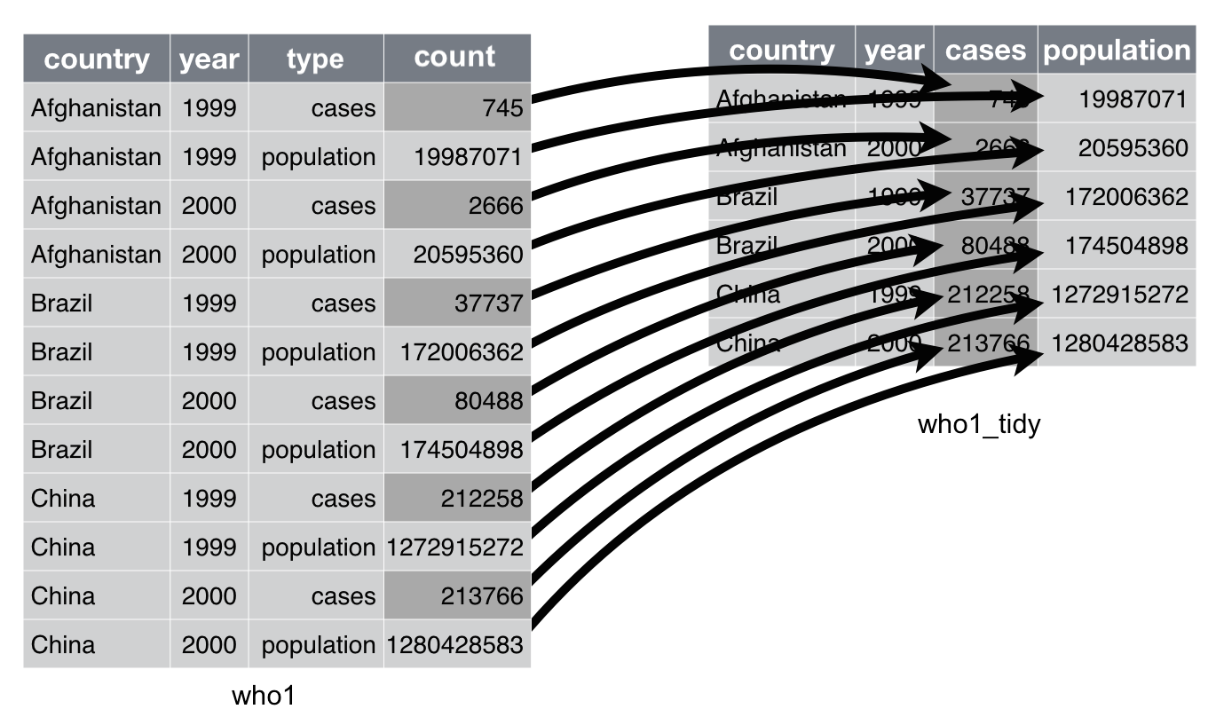
Adapted from Chapter 12 of “R for Data Science”
We can do this with function spread()as follows:
who1_tidy <- who1 %>%
   spread(value = count, key = type)
who1_tidy
## # A tibble: 6 x 4
## country year cases population
## <chr> <dbl> <int> <int>
## 1 Afghanistan 1999. 745 19987071
## 2 Afghanistan 2000. 2666 20595360
## 3 Brazil 1999. 37737 172006362
## 4 Brazil 2000. 80488 174504898
## 5 China 1999. 212258 1272915272
## 6 China 2000. 213766 1280428583Note the syntax used to tidy up who1:
- Choose a variable name to store the tidy data (this could very well be
who1again). - Use the assignment operator
<-. - Specify the variable that we want to tidy up.
- Use the pipe operator %>% to channel the contents of
who1to functionspread(more on the pipe operator later in this Part). - Invoke function
spread()and specify the column containing the values that we want to spread and the column containing the new variable names (known as the key column).
3.3.2 Gathering
You use function gather() for Problem 2: one feature is spread across multiple columns. That’s exactly the problem we saw in, for example, table who_cases from the Excel file who_split.xlsx:
who_cases## # A tibble: 3 x 3
## country `1999` `2000`
## <chr> <dbl> <dbl>
## 1 Afghanistan 745. 2666.
## 2 Brazil 37737. 80488.
## 3 China 212258. 213766.The column names 1999 and 2000 are values of the variable year, which means that each row represents two observations instead of one.
To tidy this dataset, we need to gather columns 1999 and 2000 into a new pair of variables:
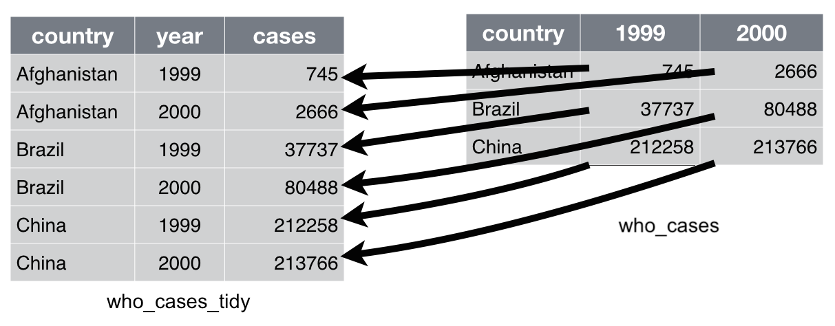
Adapted from Chapter 12 of “R for Data Science”
We can do this with function gather()as follows:
who_cases_tidy <- who_cases %>%
   gather(`1999`, `2000`, key = "year", value = "cases")
who_cases_tidy
## # A tibble: 6 x 3
## country year cases
## <chr> <chr> <dbl>
## 1 Afghanistan 1999 745.
## 2 Brazil 1999 37737.
## 3 China 1999 212258.
## 4 Afghanistan 2000 2666.
## 5 Brazil 2000 80488.
## 6 China 2000 213766.Note the syntax used to tidy up who_cases:
- Choose a variable name to store the tidy data (this could very well be
who_casesagain). - Use the assignment operator
<-. - Specify the variable that we want to tidy up.
- Use the pipe operator %>% to channel the contents of
who_casesto functiongather. - Invoke function
gather()and specify the columns we want to merge, the name of the column that will contain the merged keys and the name of the column that will contain the value for the number of tuberculosis cases per country.
3.3.3 Exercise 3.4
Consider the following tibble, which records heights and weights of 3 students:
(students <- tibble(name = rep(c("Jonas", "Ines", "Hanna"), each = 2),
                   type = rep(c("height", "weight"), 3),
                   measure = c(1.83, 81, 1.75, 71, 1.69, 55)))
## # A tibble: 6 x 3
## name type measure
## <chr> <chr> <dbl>
## 1 Jonas height 1.83
## 2 Jonas weight 81.0
## 3 Ines height 1.75
## 4 Ines weight 71.0
## 5 Hanna height 1.69
## 6 Hanna weight 55.0Use the appropriate tidyr function on variable students to make it tidy.
3.3.4 Exercise 3.5
Consider the following tibble, which records the expression of 4 genes at 3 different time points:
(genes <- tibble(symbol = c("DMD", "MYOG", "MYF5", "MYOD1"),
                d00 = c(0.697, 0.844, 1.878, 1.622),
                d02 = c(1.986, 0.051, 0.887, 1.313),
                d04 = c(0.157, 0.774, 1.507, 0.628)))
## # A tibble: 4 x 4
## symbol d00 d02 d04
## <chr> <dbl> <dbl> <dbl>
## 1 DMD 0.697 1.99 0.157
## 2 MYOG 0.844 0.0510 0.774
## 3 MYF5 1.88 0.887 1.51
## 4 MYOD1 1.62 1.31 0.628Use the appropriate tidyr function on variable genes to make it tidy.
3.4 Separating and uniting
3.4.1 Separating
When one column in a dataset contains two variables, we’ll need to use function separate() to fix the issue. That’s exactly the problem we saw in table who2:
## Parsed with column specification:
## cols(
##   country = col_character(),
##   year = col_double(),
##   rate = col_character()
## )who2## # A tibble: 6 x 3
## country year rate
## <chr> <dbl> <chr>
## 1 Afghanistan 1999. 745/19987071
## 2 Afghanistan 2000. 2666/20595360
## 3 Brazil 1999. 37737/172006362
## 4 Brazil 2000. 80488/174504898
## 5 China 1999. 212258/1272915272
## 6 China 2000. 213766/1280428583Column rate contains both cases and population, so we need to split it in two:
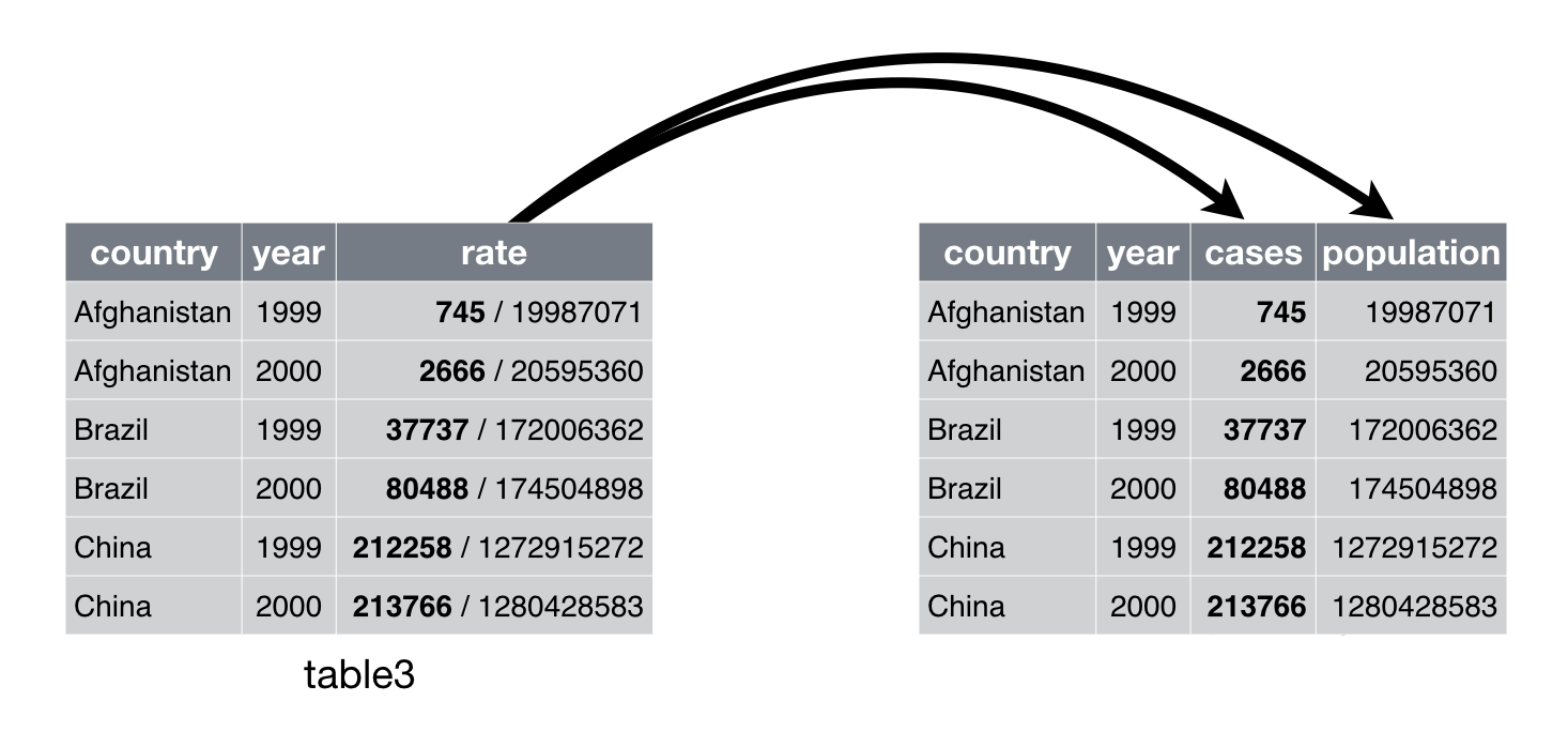
Adapted from Chapter 12 of “R for Data Science”
We can do this with function separate()as follows:
who2_tidy <- who2 %>%
   separate(rate, into = c("cases", "population"), sep = "/")
who2_tidy
## # A tibble: 6 x 4
## country year cases population
## <chr> <dbl> <chr> <chr>
## 1 Afghanistan 1999. 745 19987071
## 2 Afghanistan 2000. 2666 20595360
## 3 Brazil 1999. 37737 172006362
## 4 Brazil 2000. 80488 174504898
## 5 China 1999. 212258 1272915272
## 6 China 2000. 213766 1280428583Note the syntax used to tidy up who2:
- Choose a variable name to store the tidy data (this could very well be
who2again). - Use the assignment operator
<-. - Specify the variable that we want to tidy up.
- Use the pipe operator %>% to channel the contents of
who2to functionseparate(). - Invoke function
separate()and specify the column we want to split, the name of the new columns and the separator that is currently merging the variables.
3.4.2 Uniting
When a variable is stored in two separate columns and is more convenient to combine them, we need to use function unite(). Table who3 has this problem:
who3 <- read_tsv("datasets/who3.tsv")## Parsed with column specification:
## cols(
## country = col_character(),
## century = col_integer(),
## year = col_character(),
## rate = col_character()
## )who3## # A tibble: 6 x 4
## country century year rate
## <chr> <int> <chr> <chr>
## 1 Afghanistan 19 99 745/19987071
## 2 Afghanistan 20 00 2666/20595360
## 3 Brazil 19 99 37737/172006362
## 4 Brazil 20 00 80488/174504898
## 5 China 19 99 212258/1272915272
## 6 China 20 00 213766/1280428583Column century and year can be combined into a single column called year:
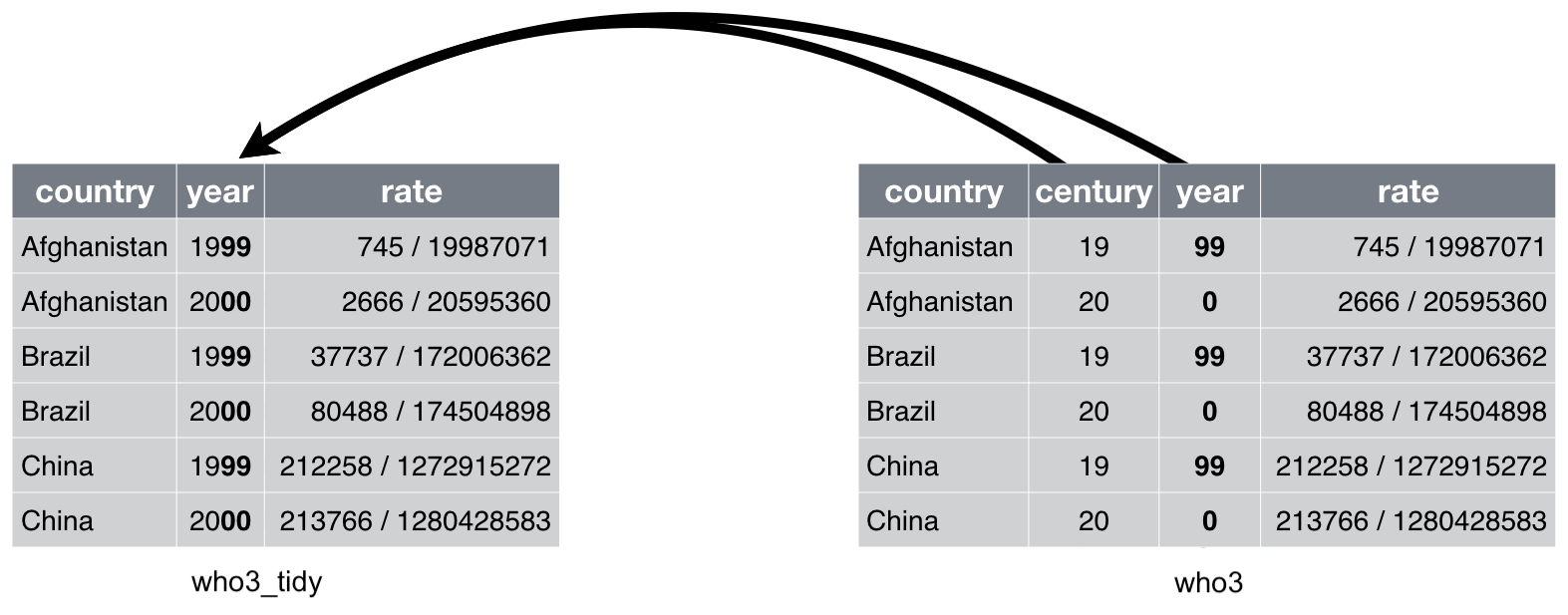
Adapted from Chapter 12 of “R for Data Science”
We can do this with function unite()as follows:
who3_tidy <- who3 %>%
   unite(century, year, col = "year", sep = "")
who3_tidy
## # A tibble: 6 x 3
## country year rate
## <chr> <chr> <chr>
## 1 Afghanistan 1999 745/19987071
## 2 Afghanistan 2000 2666/20595360
## 3 Brazil 1999 37737/172006362
## 4 Brazil 2000 80488/174504898
## 5 China 1999 212258/1272915272
## 6 China 2000 213766/1280428583Note the syntax used to tidy up who3:
- Choose a variable name to store the tidy data (this could very well be
who3again). - Use the assignment operator
<-. - Specify the variable that we want to tidy up.
- Use the pipe operator %>% to channel the contents of
who3to functionunite(). - Invoke function
unite()and specify the columns we want to merge, the name of the new column and the separator that we want to use to merge the column values.
3.4.3 Exercise 3.6
Consider the following tibble, which records heights and weights of 3 students:
(students <- tibble(name = c("Jonas", "Ines", "Hanna"),
                   ratio = c("81/1.83", "71/1.75", "55/1.69")))
## # A tibble: 3 x 2
## name ratio
## <chr> <chr>
## 1 Jonas 81/1.83
## 2 Ines 71/1.75
## 3 Hanna 55/1.69Use the appropriate tidyr function on variable students to make it tidy.
3.4.4 Exercise 3.7
Consider the following tibble, which records the price of 4 drugs:
(drugs <- tibble(name = c("penicillin", "insuline", "aspirin", "lanoxin"),
                euros = c(13, 17, 5, 25),
                cents = c(81, 20, 14, 12)))
## # A tibble: 4 x 3
## name euros cents
## <chr> <dbl> <dbl>
## 1 penicillin 13. 81.
## 2 insuline 17. 20.
## 3 aspirin 5. 14.
## 4 lanoxin 25. 12.Use the appropriate tidyr function on variable drugs to make it tidy.
3.5 The %>% operator
As you know already, we channel the contents of a tibble to the different tidyr functions using the pipe operator: %>%.
Pipes are a powerful tool for clearly expressing the operation we want to perform on a variable. In addition, they can be used to apply a sequence of operations to a variable.
Table who3, for example, has two problems: cases and population are expressed as a rate and year is split in columns century and year:
who3## # A tibble: 6 x 4
## country century year rate
## <chr> <int> <chr> <chr>
## 1 Afghanistan 19 99 745/19987071
## 2 Afghanistan 20 00 2666/20595360
## 3 Brazil 19 99 37737/172006362
## 4 Brazil 20 00 80488/174504898
## 5 China 19 99 212258/1272915272
## 6 China 20 00 213766/1280428583So, we clearly need two steps to tidy up this dataset:
who3_tidy <- who3 %>%
   separate(rate, into = c("cases", "population"), sep = "/")

who3_tidy <- who3_tidy %>%
   unite(century, year, col = "yyyy", sep = "")

who3_tidy
## # A tibble: 6 x 4
## country yyyy cases population
## <chr> <chr> <chr> <chr>
## 1 Afghanistan 1999 745 19987071
## 2 Afghanistan 2000 2666 20595360
## 3 Brazil 1999 37737 172006362
## 4 Brazil 2000 80488 174504898
## 5 China 1999 212258 1272915272
## 6 China 2000 213766 1280428583Thanks to the pipe, we can apply these two operations to who3 in one go:
who3_tidy <- who3 %>%
  separate(rate, into = c("cases", "population"), sep = "/") %>%
  unite(century, year, col = "yyyy", sep = "")

who3_tidy
## # A tibble: 6 x 4
## country yyyy cases population
## <chr> <chr> <chr> <chr>
## 1 Afghanistan 1999 745 19987071
## 2 Afghanistan 2000 2666 20595360
## 3 Brazil 1999 37737 172006362
## 4 Brazil 2000 80488 174504898
## 5 China 1999 212258 1272915272
## 6 China 2000 213766 1280428583Note that this process reads almost like natural language:
- We channel (or pipe) the contents of
who3to functionseparate(). separate()splits columnrateinto columnscasesandpopulationusing “/” as separator.- The result of
separate()is piped to functionunite(). unite()combines columnscenturyandyearinto columnyyyyusing the blank character as separator.
Even though writing the above code on a single line of code is still valid, it is good practice to use ENTER (i.e. a new line) after every %>% for clarity.